Build A Distributed Tiling Pipeline
Overview
Problem solved: turn a directory of whole-slide images into a scalable tile dataset that can be filtered and saved for model training or large-batch inference.
Use this pipeline when:
- you need dense tile extraction,
- you want to keep slide metadata and tile metadata in Ray,
- and you only want to read pixels at the point where they become necessary.
Workflow
- Read slide metadata with
read_slides. - Add a stable slide identifier.
- Expand each slide into tile coordinates with
grid_tiles. - Repartition tiles for better parallelism.
- Read tile pixels with
read_slide_tiles. - Filter tiles and write the result.
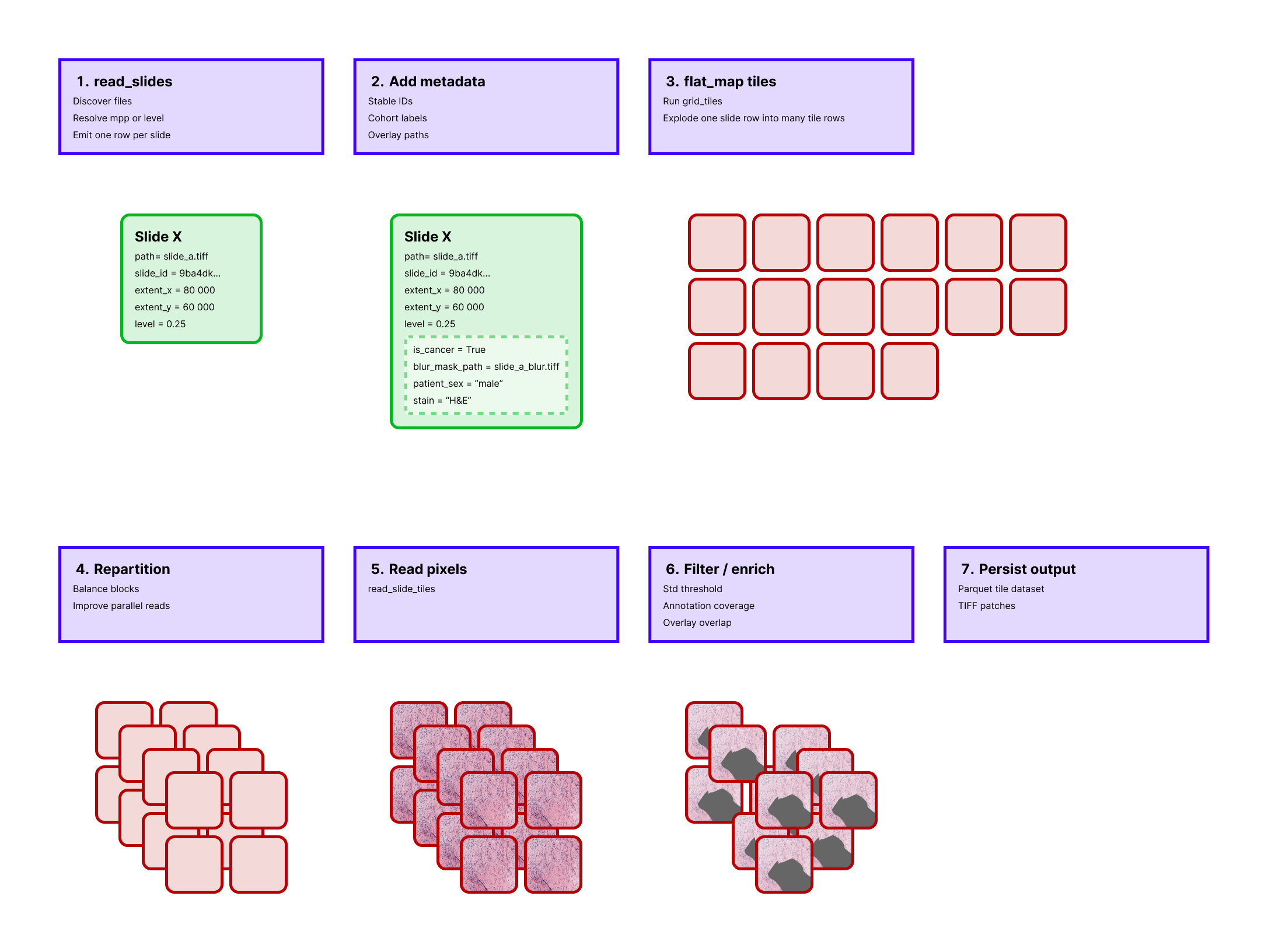 The pipeline stays metadata-only until tile pixels are actually needed, which is why it scales better than eager extraction.
Example
from typing import Any

from ray.data.expressions import col

from ratiopath.ray import read_slides
from ratiopath.tiling import grid_tiles, read_slide_tiles
from ratiopath.tiling.utils import row_hash


def expand_tiles(row: dict[str, Any]) -> list[dict[str, Any]]:
    return [
        {
            "tile_x": x,
            "tile_y": y,
            "path": row["path"],
            "slide_id": row["id"],
            "level": row["level"],
            "tile_extent_x": row["tile_extent_x"],
            "tile_extent_y": row["tile_extent_y"],
        }
        for x, y in grid_tiles(
            slide_extent=(row["extent_x"], row["extent_y"]),
            tile_extent=(row["tile_extent_x"], row["tile_extent_y"]),
            stride=(row["stride_x"], row["stride_y"]),
            last="keep",
        )
    ]


slides = read_slides("data", mpp=0.25, tile_extent=1024, stride=960)
slides = slides.map(row_hash, num_cpus=0.1, memory=128 * 1024**2)

tiles = slides.flat_map(expand_tiles, num_cpus=0.2, memory=128 * 1024**2)
tiles = tiles.repartition(target_num_rows_per_block=128)

tiles_with_pixels = tiles.with_column(
    "tile",
    read_slide_tiles(
        col("path"),
        col("tile_x"),
        col("tile_y"),
        col("tile_extent_x"),
        col("tile_extent_y"),
        col("level"),
    ),
    num_cpus=1,
    memory=4 * 1024**3,
)

tissue_tiles = tiles_with_pixels.filter(lambda row: row["tile"].std() > 8)
tissue_tiles.write_parquet("tiles")
Under the hood
This pipeline is intentionally staged so that expensive operations happen as late as possible.
read_slides produces one row per slide.
row_hash adds a stable identifier.
flat_map with grid_tiles explodes each slide into many metadata-only tile rows.
repartition then redistributes those rows so later pixel reads do not remain concentrated in the same original block.
Only after that does read_slide_tiles open slide files and decode image regions.
Internally, the reader groups rows by slide path so a batch can reuse the same backend handle and avoid unnecessary reopen overhead.
The final filter is just one example of a metadata-plus-pixels decision rule. In a production pipeline, you can replace it with overlay coverage, annotation coverage, or a model-based triage stage.
Why This Pipeline Works Well
- metadata stays compact until tile pixels are required,
- slide reads are grouped by source path inside the tile reader,
- and Ray can schedule different stages with different resource hints.
Useful Variants
- replace the simple standard-deviation filter with an overlay-based tissue mask,
- switch from
mpptolevelif your workflow is pyramid-level specific, - or persist the slide-level metadata table separately for reproducibility.
Why the metadata table is worth keeping
Persisting the slide-level table separates slide discovery and level resolution from downstream tile extraction. That gives you a reproducible snapshot of exactly which files, scales, and tile settings were used to generate a dataset.
It also makes later pipeline reruns cheaper because you can restart from normalized slide metadata instead of repeating the initial scan over raw slide files.